R Shiny Basics

Alissa Gordon

Learning Goals:

Know what a Shiny App is and why it is useful
Be able to differentiate between what goes in the UI versus the server
Use inputs, outputs, and reactive coding to create your own shiny app

What is a shiny app?

Shiny

Shiny is an R package that allows us to build and share interactive web applications through R. If you do not already have it, go ahead and install the following packages:

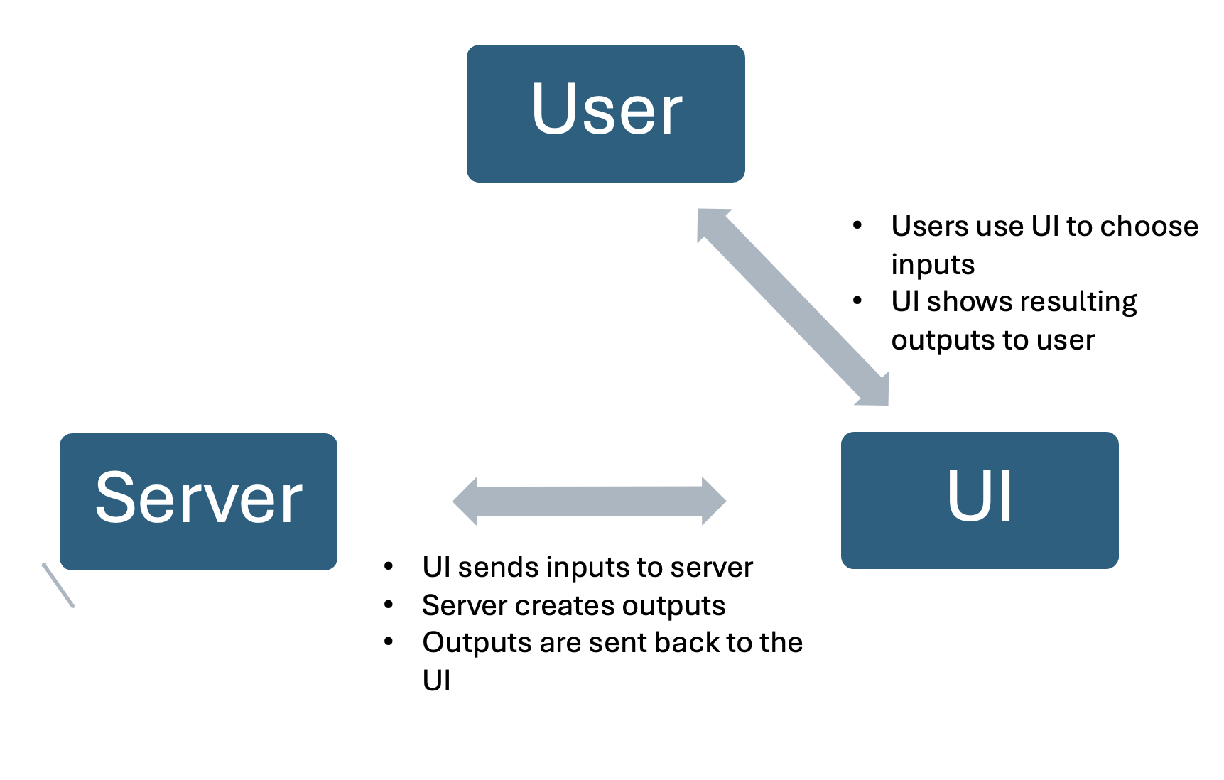
install.packages('shiny')
install.packages('shinyWidgets')

Why are shiny apps useful?

They are useful because…

We can make complex apps without knowledge of languages such as HTML and JavaScript
We can share them easily as R files for local implementation or as URLs
They are open source (affordable and accessible)!
They allow for interactive and quick data exploration

What is the basic structure of a shiny app?

Shiny structure

Shiny apps consist of two key components, both coded in R!
These components are the User Interface (aka UI) and the Server
These two work together, communicating through inputs and outputs, to create the shiny app

The UI and Server

The UI is the front-end of a Shiny app, where users interact with various input elements (like sliders, buttons, text fields, and dropdowns). It defines what the app looks like and how users provide their preferences or data.
These preferences are processed by the server. The server performs the necessary computations, and generates outputs (such as plots and tables).
These outputs are then sent back to the UI to be displayed to the users!

The Restaurant Analogy: The UI

In the grand scheme of the shiny app, you can think of the shiny app as a restaurant.
The user of the shiny app is the restaurant customer, and the UI is the table where the customer sits at! You can also think of the user inputs as a dinner menu at the restaurant, giving the customer different options for their food.

The Restaurant Analogy: The Server

The customer’s orders are then taken back to the kitchen. We can think of the kitchen and staff as our shiny server. You can think of the meal as the output from the shiny app. The kitchen makes the customer’s meal based on their order.

The Restaurant Analogy: Back to the UI!

Once the meal is created, it is brought back to the customer’s table for the customer to enjoy!
For the restaurant to be successful, we want to ensure proper communication between the customer and the kitchen so that the customer gets what they want!

Summary

The UI and the server work closely together to create the shiny app.
The shiny app works like a restaurant. If the customers’ orders are not properly communicated to the kitchen, we will have wrong orders and unhappy customers!

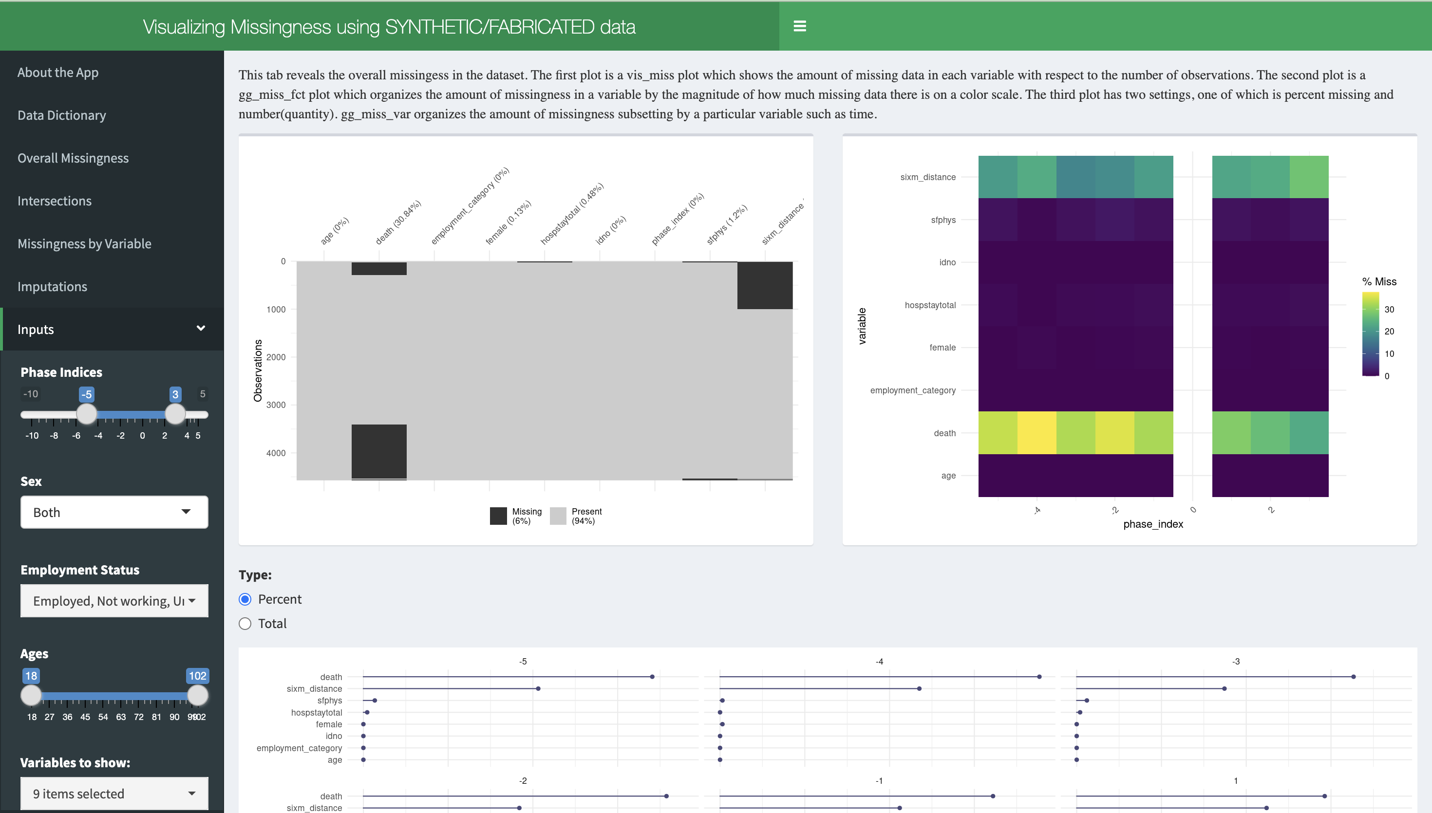
Learning Check

Why are shiny apps useful?
What are the two main components of a shiny app, and what do they do?
Fill in the blanks: The inputs are selected in the _____ by the app users. The outputs are then created in the ________ and later shown back in the _________.

How do we work with inputs and outputs?

Inputs

Inputs are displayed on the UI for users to choose different options for their analysis.
With inputs, we can select variables, filter data, change plot types, and more!
Luckily, we have ‘widgets’ that are easy functions to create inputs through shinyWidgets and other similar packages.
When you list inputs in the UI, be sure to separate them with commas

Input Structure

The basic structure of input functions are similar to each other.

The key to using inputs is to properly ID them so we can call them throughout our server code. We call them with ‘input$inputId’ in our code.

Example input function

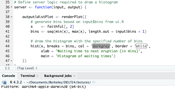
Creating Outputs

Outputs can be a range of objects including but not limited to tables, graphs, and text.
Whenever we create output in the server, we make code them inside ‘render’ functions. Rendering is the process of converting code into a format that can be displayed and interacted with by users.
In our restaurant analogy, we can think of the raw code to create the outputs as ingredients. These must be cooked before we can serve them, so we can think of rendering as cooking our ingredients.

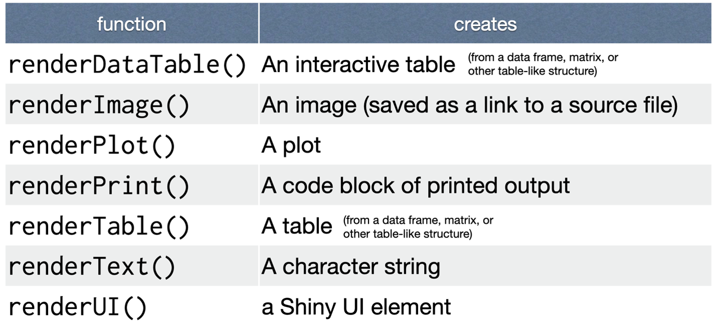
Common render functions

Output Structure

The basic structure when rendering outputs are also similar to one another.
The key to using outputs is to properly ID them so we can call them back to our UI. We name them in the server with ‘output$outputID’.
We also want to make sure that we are using the correct render function based on our desired output.

output$myoutputid<-renderPlot({
  hist(xvar)
})

Calling our outputs

We can call our outputs back to our UI by using their output IDs.
We have code that allows us to call outputs based on their output type.

plotOutput("myoutputid")

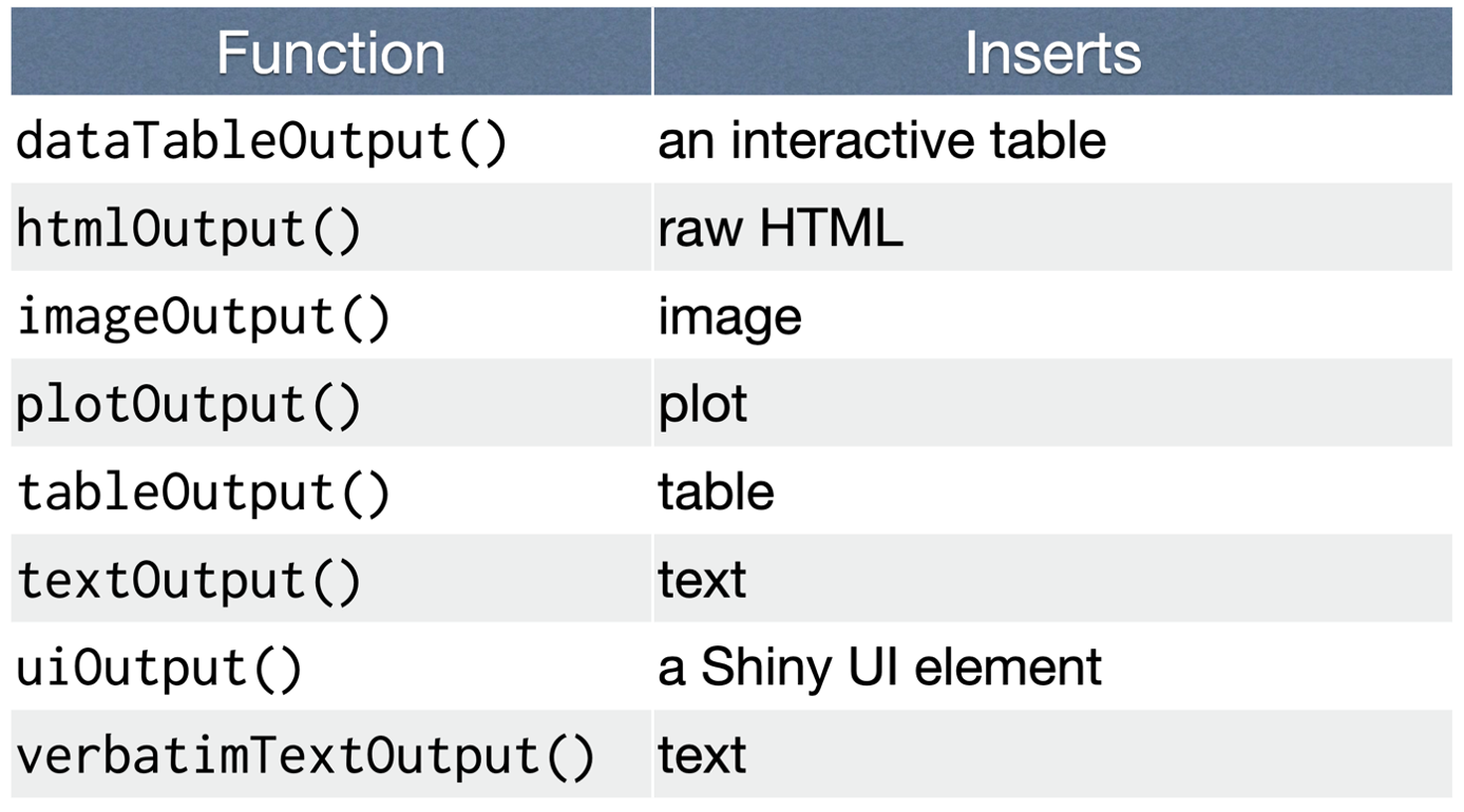
Common output functions

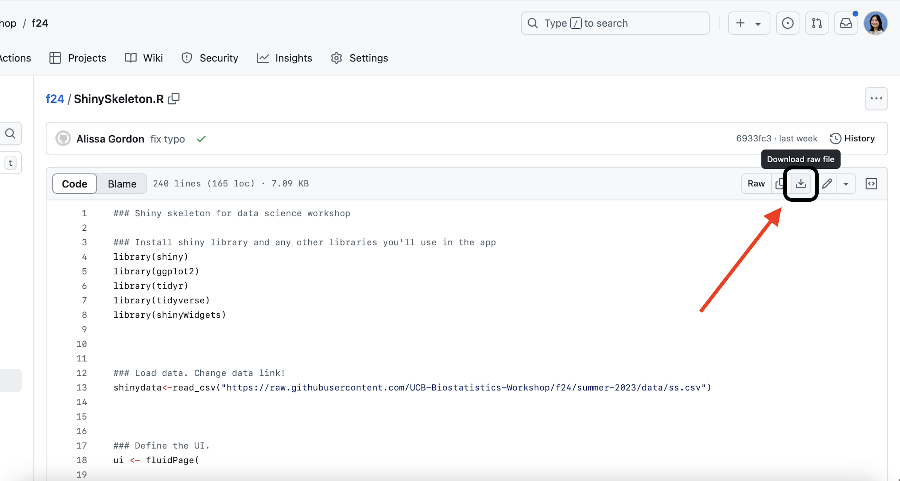
A note on the reactive function

You will see code later that uses the reactive function in the server. The main thing to know about the reactive function is that it allows us to streamline our computations. For example, say we filter all of our data based on a single value. Instead of repeating this computation within every render function, we can filter our data in the reactive function. We can then use the data from the reactive function throughout the server. This allows us to only perform the computation once instead of in every render function.

Exercises: Labeling our inputs and outputs!

What does the following piece of code do? Address all arguments in the function.

selectInput("myselection", label=h3("Selection Box"),
            choices=list("First"=1, "Second"=2, "Third"=3),
            selected=2)

What is wrong with the following pieces of code? How would you fix it?
a.

myplot<-renderPlot(
  hist(x)
)

tableOutput(myoutputtable)

How do we deploy our apps?

Local versus Hosted

One of the great things about shiny apps is that we can deploy them locally (on our own computers) or host them online (with URLs anyone can access). Deploying our apps locally doesn’t necessarily mean no one else can access them since we can share the code for people to also locally deploy the shiny app. For now we will focus on local deployment.

We can locally deploy the app just by running the shinyApp function after defining the UI and the server!
This will pop up a separate window with your functional shiny app
If there are any errors in the UI or server code, your app will not run or will not run as expected

ui<-fluidPage(
  
)

server<-function(input, output){
  
}

shinyApp(ui = ui, server = server)

Demo time!

Shiny Skeleton Code

If you don’t already have the shiny skeleton code for the demo, go ahead and download it!

Project time!

Project Description

Working in small groups, create your own Shiny app using the Shiny Skeleton!

Choose one of the three data set options
Explore the data set to find two interesting trends in the data between different variables
Include two different types of plots in your app
Include one filtering option in your app
Write a few bullet points about your findings
At the end, you will present your app to the whole group :)

Project Datasets: Heart Disease

heart_disease = read_csv("https://bit.ly/ucb_biostat_heart_disease_data")
head(heart_disease)

# A tibble: 6 × 9
   ...1   age   sex blood_pressure cholesterol fbs_over_120 max_hr
  <dbl> <dbl> <dbl>          <dbl>       <dbl>        <dbl>  <dbl>
1     1    70     1            130         322            0    109
2     2    80     0            115         564            0    160
3     3    55     1            124         261            0    141
4     4    65     1            128         263            0    105
5     5    45     0            120         269            0    121
6     6    30     1            120         177            0    140
# ℹ 2 more variables: exercise_angina <dbl>, heart_disease <chr>

Project Datasets: Marketing Campaign

marketing = read_csv("https://bit.ly/ucb_biostat_marketing_data")
head(marketing)

# A tibble: 6 × 12
   ...1    id birth_year education  marital_status income fruit_purchases
  <dbl> <dbl>      <dbl> <chr>      <chr>           <dbl>           <dbl>
1     1  5524       1957 Graduation Single          58138              88
2     2  2174       1954 Graduation Single          46344               1
3     3  4141       1965 Graduation Together        71613              49
4     4  6182       1984 Graduation Together        26646               4
5     5  5324       1981 PhD        Married         58293              43
6     6  7446       1967 Master     Together        62513              42
# ℹ 5 more variables: meat_purchases <dbl>, fish_purchases <dbl>,
#   candy_purchases <dbl>, sale_purchases <dbl>, complaint <dbl>

Project Datasets: Student Achievement Data

student = read_csv("https://bit.ly/ucb_biostat_student_data")
student = student[sample(nrow(student), size=500),]
head(student)

# A tibble: 6 × 14
   ...1 student_id hours_studied attendance parental_involvement
  <dbl>      <dbl>         <dbl>      <dbl> <chr>               
1  6248       6248            24         76 High                
2  5420       5420            13         65 Low                 
3  2768       2768            23         67 Medium              
4  6527       6527            18         91 Low                 
5  4383       4383            16         67 Medium              
6  1817       1817             7         92 High                
# ℹ 9 more variables: access_to_resources <chr>, sleep_hours <dbl>,
#   previous_scores <dbl>, internet_access <chr>, family_income <chr>,
#   teacher_quality <chr>, school_type <chr>, gender <chr>, exam_score <dbl>